Force Model¶

The satkit numerical propagator integrates the forces acting on a satellite to produce a change in velocity, then integrates the velocity to produce a change in position:

\[ \vec{v}(t_1)~=~\vec{v}(t_0) + \int_{t_0}^{t_1}~\vec{a}\left ( t,~\vec{p}_{t},~\vec{v}_{t} \right ) ~dt \]

\[ \vec{p}(t_1)~=~\vec{p}(t_0) + \int_{t_0}^{t_1}~\vec{v}(t)~dt \]

This page describes each force in \(\vec{a}\left (t, \vec{p}, \vec{v}\right )\) that satkit models. The integration mechanics live in the ODE Integrators page; state vectors, the state transition matrix, and covariance propagation live in State Vectors, STM & Covariance.

The force model follows the treatment in Montenbruck & Gill (2000), Satellite Orbits: Models, Methods, Applications, Chapter 3 — consult that book for more depth on any term. Every model below cites its primary source; the full list is on the References page.

Summary¶

Force	Default	Setting	Order of magnitude (LEO)
Earth gravity (spherical harmonics)	on	`gravity_degree`, `gravity_order`, `gravity_model`	\(10^0\) m/s²
Sun third-body	on	`use_sun_gravity`	\(10^{-6}\) m/s²
Moon third-body	on	`use_moon_gravity`	\(10^{-6}\) m/s²
Atmospheric drag (NRLMSISE-00)	when alt < 700 km	`use_spaceweather`, `satproperties.cd_a_over_m`	\(10^{-7}\) to \(10^{-3}\) m/s²
Solar radiation pressure (cannonball)	when `craoverm > 0`	`satproperties.craoverm`	\(10^{-8}\) to \(10^{-7}\) m/s²
Solar radiation pressure (ECOM, experimental — see Empirical SRP: ECOM)	when `ecom` is set	`satproperties.ecom`	\(10^{-7}\) m/s² (D0), \(10^{-9}\) (Y, B)
Solid Earth tides (IERS 2010 §6.2.1 Step 1)	on	`tide_model`	\(10^{-7}\) m/s²
General relativity (IERS 2010 §10.3: Schwarzschild + geodesic + Lense–Thirring)	on	`use_relativistic_correction`	\(10^{-9}\) m/s² (LEO)
Continuous thrust	when configured	`satproperties.thrusts`	user-specified

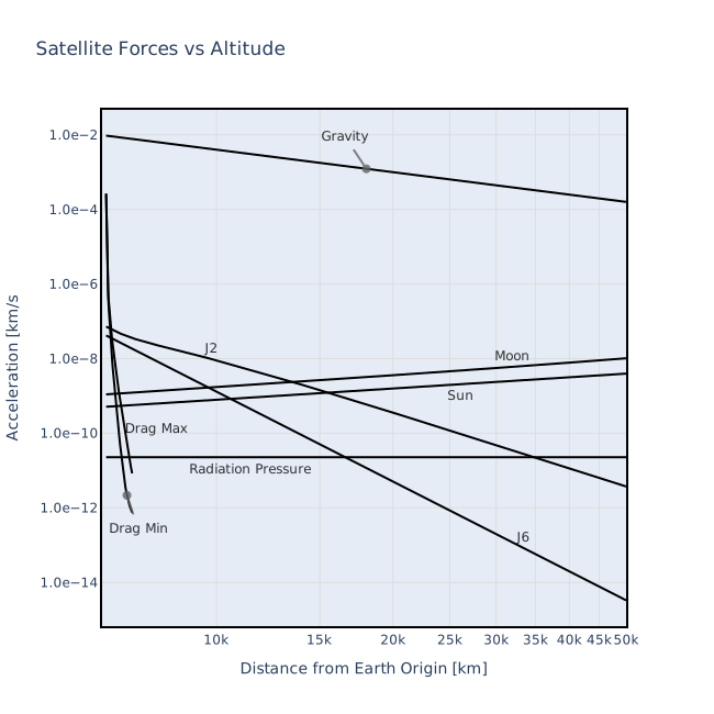
The Forces-vs-altitude plot at the bottom of this page shows how each contribution scales with orbital altitude.

Earth Gravity¶

Earth's gravity dominates by many orders of magnitude. The Earth is not a point mass; its non-spherical mass distribution is captured by an expansion in spherical harmonics with coefficients \(\bar{C}_{nm}, \bar{S}_{nm}\):

\[ V(r, \phi, \lambda) = \frac{GM_\oplus}{r}\sum_{n=0}^{N}\left(\frac{R_\oplus}{r}\right)^n \sum_{m=0}^{n} \bar{P}_{nm}(\sin\phi)\left[\bar{C}_{nm}\cos m\lambda + \bar{S}_{nm}\sin m\lambda\right] \]

The \(\bar{C}_{20}\) term (commonly called J2) captures Earth's equatorial bulge and is responsible for orbital precession. The expansion and the recursive evaluation of the normalized Legendre functions follow Montenbruck & Gill (2000), §3.2, Eqs. 3.28–3.33.

Coefficient files come from ICGEM (Ince et al. 2019). satkit ships with four models, selectable via gravity_model:

Model	Description
`egm96`	Earth Gravitational Model 1996 (default) — Lemoine et al. (1998); tide-free
`jgm3`	Joint Gravity Model 3 — Tapley et al. (1996); zero-tide
`jgm2`	Joint Gravity Model 2 — Nerem et al. (1994); zero-tide
`itugrace16`	ITU_GRACE16 — Akyilmaz et al. (2016); zero-tide

The gravity_degree and gravity_order parameters cap the expansion (default 4×4). For high-precision work, degree-8 to degree-20 is typical; gains beyond ~degree-20 are small for satellites above ~500 km (satkit's recommendation — see the order-of-magnitude discussion of gravity-model truncation in Montenbruck & Gill 2000, §3.2). Order may be set lower than degree to zero out the longitudinal (tesseral) terms.

Third-Body Gravity (Sun, Moon)¶

The Sun and Moon each act as point-mass attractors. Their pull on the Earth must be subtracted to express acceleration in the geocentric frame:

\[ \vec{a}_\text{sun}~=~GM_\text{sun}\left[\frac{\vec{p}_\text{sun} - \vec{p}}{|\vec{p}_\text{sun}-\vec{p}|^3} - \frac{\vec{p}_\text{sun}}{|\vec{p}_\text{sun}|^3}\right] \]

The Moon expression has the same form (Montenbruck & Gill 2000, §3.3.1, Eq. 3.37). Body positions come from the JPL DE-series ephemerides (default DE440; Park et al. 2021). Disable either with use_sun_gravity=False / use_moon_gravity=False.

Solid Earth Tides¶

The Sun and Moon deform the solid body of the Earth, which in turn perturbs the geopotential. satkit implements IERS 2010 §6.2.1 Step 1 (Petit & Luzum 2010, Eqs. 6.6–6.7, with the anelastic Love numbers of Table 6.3) — the frequency-independent Love-number response, which in satkit's own measurements carries about 99% of the total solid-tide signal at ~5% per-step CPU overhead. The correction modifies the degree-2, degree-3, and a small degree-4 set of Stokes coefficients \(\Delta\bar{C}_{nm}, \Delta\bar{S}_{nm}\) as a function of Sun and Moon ITRF positions and the IERS 2010 nominal Love numbers.

Frequency-dependent corrections (IERS 2010 §6.2.2 Step 2, Tables 6.5a–c, 71 tidal constituents) are reserved for TideModel::SolidFull — currently a placeholder that falls back to Step 1. The Step 2 contribution is sub-mm class at LEO.

Set with tide_model:

Value	Effect
`tidemodel.solid_step1` (default)	IERS §6.2.1 Step 1 — recommended
`tidemodel.solid_full`	Step 1 + Step 2 (Step 2 not yet implemented; behaves as Step 1)
`tidemodel.none`	Disable solid tides (use for reproducibility with pre-tide versions)

Tide system of the gravity model

Step 1 includes the permanent tide, so it belongs on a tide-free gravity model. gravmodel.egm96 (the default) is tide-free (\(\bar{C}_{20} = -4.84165371736\times10^{-4}\)); gravmodel.jgm3 and gravmodel.itugrace16 are zero-tide (\(\bar{C}_{20} \approx -4.841695\times10^{-4}\)), so combining them with solid_step1 double-counts the permanent tide — about 5–7 cm cross-track over 3 days at GPS altitude. Use egm96 with tides on, or tidemodel.none with a zero-tide model.

Atmospheric Drag¶

At altitudes below 700 km the residual atmosphere imposes a drag force:

\[ \vec{a}_\text{drag}~=~-\frac{1}{2}\,C_d\frac{A}{m}\,\rho\,|\vec{v}_r|\vec{v}_r \]

with \(C_d\) the drag coefficient (typically 1.5–3; Montenbruck & Gill 2000, §3.5), \(A/m\) the area-to-mass ratio, \(\rho\) the atmospheric density, and \(\vec{v}_r\) the satellite velocity relative to the co-rotating atmosphere (assumed at rest in the Earth-fixed frame).

Density comes from the NRLMSISE-00 thermosphere model (Picone et al. 2002; a pure-Rust port of Dominik Brodowski's C implementation), which reads the space-weather indices from the CelesTrak SW-All.csv table automatically, following the model's own interface: the observed F10.7 of the previous UTC day, the observed 81-day centred average F10.7A of the current day, and the 7-element 3-hourly geomagnetic history (the current day's daily Ap, the current 3-hourly ap and the three before it, and the 12–33 h and 36–57 h means — NRLMSISE-00 switch 9 = −1), which lets the density respond to a geomagnetic storm within hours rather than at the next UTC midnight. When that history cannot be assembled (a day missing from the table, or a monthly predicted row without 3-hourly values) the model falls back to the current day's daily Ap. Disable space-weather lookup with use_spaceweather=False to fall back to fixed nominal indices (F10.7 = F10.7A = 150, Ap = 4).

Drag is skipped above 700 km regardless of settings.

Solar Radiation Pressure¶

Solar photons absorbed or scattered by the satellite transfer momentum, producing a force away from the Sun:

\[ \vec{a}_\text{SRP}~=~-P_\text{sun}\,C_R\frac{A}{m}\,\hat{p}_\text{sun} \cdot \nu(\vec{p}, \vec{p}_\text{sun}) \]

where \(P_\text{sun} \approx 4.56 \times 10^{-6}\) N/m² is the radiation pressure at 1 AU, \(C_R A/m\) is the satellite's radiation susceptibility (the user-supplied satproperties.craoverm), and \(\nu(\vec{p}, \vec{p}_\text{sun}) \in [0, 1]\) is a shadow function that vanishes when the satellite is in Earth's umbra — the conical umbra/penumbra model of Montenbruck & Gill (2000), §3.4.2; the cannonball force itself is their §3.4, Eq. 3.75.

satkit's default is a cannonball model — the satellite's surface is treated as if its normal points toward the Sun, and the force acts along the satellite→Sun line. A physical box-wing model (Rodriguez-Solano et al. 2012) is not provided.

For GNSS-class work satkit also offers the Empirical CODE Orbit Model (ECOM) — the empirical, Sun-oriented D/Y/B parameterization used by CODE and most IGS analysis centres — as an experimental addition to the cannonball term, enabled by supplying coefficients through satproperties(ecom=...). Its equations, coefficient table, sign and eclipse conventions, and measured performance are on the Empirical SRP: ECOM page.

Moon geometry and quadruples the fit residual. And for arcs that cross Earth's shadow, use integrator = gauss_jackson8: the adaptive Runge–Kutta steppers can abort at a shadow boundary with too many consecutive step rejections, whereas the fixed-step multistep integrator is immune and fits an eclipsing satellite just as well (G08, 8% umbra: 4.7 cm fit, 5.6 cm at 24 h).

General-Relativistic Correction¶

The full IERS 2010 §10.3 Eq. 10.12 correction (Petit & Luzum 2010) with PPN parameters \(\beta = \gamma = 1\), three terms:

\[ \vec{a}_\text{GR}~=~\underbrace{\frac{GM_\oplus}{c^2 r^3}\left[\left(\frac{4GM_\oplus}{r} - v^2\right)\vec{r} + 4(\vec{r}\cdot\vec{v})\vec{v}\right]}_\text{Schwarzschild} ~+~\underbrace{2\,\vec{\Omega}\times\vec{v}}_\text{geodesic} ~+~\underbrace{\frac{2GM_\oplus}{c^2 r^3}\left[\frac{3}{r^2}(\vec{r}\times\vec{v})(\vec{r}\cdot\vec{J}) + \vec{v}\times\vec{J}\right]}_\text{Lense–Thirring} \]

where \(\vec{\Omega} = \tfrac{3}{2}\,\frac{GM_\odot}{c^2 R_\oplus^3}\,(\vec{R}_\oplus\times\dot{\vec{R}}_\oplus)\) is the geodesic (de Sitter) precession of the geocentric frame from the Earth's heliocentric state \(\vec{R}_\oplus, \dot{\vec{R}}_\oplus\) (\(|\Omega| \approx 1.92''\)/century), and \(\vec{J} = \tfrac{2}{5}R^2\omega\,\hat{z}_\text{ITRF}\) is the Earth's spin angular momentum per unit mass (homogeneous rigid-sphere approximation, \(\approx 1.19\times10^9\) m²/s; the real moment-of-inertia factor is ≈0.33 rather than 0.4, a ~20% overstatement of a term that is ≤\(10^{-10}\) m/s² and mostly periodic — GMAT uses the same approximation, GMAT Mathematical Specifications, §4.2.6).

The Schwarzschild term dominates below GEO (~\(10^{-9}\) m/s² at LEO; in satkit runs, omitting it costs ~1 m/day at GPS altitude and ~3 m/day at GEO). The geodesic term is a near-constant \(4\times10^{-11}\) m/s² Coriolis-like acceleration at LEO and becomes the largest relativistic term beyond ~100,000 km (~1 m over 7 days at 200,000 km, measured in the GMAT comparison). Lense–Thirring is ~\(10^{-10}\) m/s² at LEO, mostly periodic, and falls as \(1/r^3\). This is the same formulation as GMAT's RelativisticCorrection (GMAT Mathematical Specifications, §4.2.6).

Toggle with use_relativistic_correction (default True).

Continuous Thrust¶

Constant acceleration in a chosen frame (used to model low-thrust maneuvers or — in orbit-determination contexts — empirical accelerations: a fitted catch-all that absorbs un-modeled physics). See satkit.thrust and the GPS Example tutorial for usage.

Future Propagation¶

When propagating into the future beyond the date range of downloaded data files:

Earth Orientation Parameters (\(\Delta UT1\), \(x_p\), \(y_p\)): the last available values are held constant, with a one-time warning. This is much more accurate than defaulting to zero, but still drifts by ~0.1″ / ~10 ms over a few months (metres at LEO); check satkit.frametransform.eop_status(t) or set propsettings.require_eop_coverage = True to make the propagator raise instead, and refresh with satkit.utils.update_datafiles(). A propagation with no EOP table loaded at all is refused.
Space Weather (F10.7 solar flux, Ap geomagnetic index): if historical data isn't available, the NOAA/SWPC solar cycle forecast supplies predicted F10.7 (out ~5 years). Ap defaults to 4. If neither source is available, F10.7 = 150 and Ap = 4 are used. Run satkit.utils.update_datafiles() to refresh both.

Forces vs Altitude¶

The plot below, modeled on Fig. 3.1 of Montenbruck & Gill (2000), shows each force's order of magnitude vs orbital altitude:

Acceleration vs Altitude